I/O Characterisitcs of Microsoft SQL Server – Part I
June 28, 2016 Leave a comment
Database happens to be one of most common applications running in data centers. Anytime, you think of storing data for later use, you will have to consider some form of data management systems for doing so. Database is one such data management systems offering sophisticated mechanisms to store, access, and protect data. Various queries can be run against the database to retrieve data at various granularity (individual data record, groups of records or all the data in a database).
Databases are available in many flavors – Commercial: Oracle, Microsoft SQL Server, IBM DB2, Open Source: PostGreSQL, MySQL. Irrespective of the flavor, goal of a database is the same – save data for later consumption. With databases becoming the conduit for accessing / storing data and the amount of data they have to handle exploding to insane proportions, it was necessary to redesign IT infrastructure supporting these data management systems. Separating the storage tier from compute tier gave architects a lot of flexibility when designing and managing the infrastructure for these systems. Storing the data managed by a database in a separate layer offers interesting new possibilities – design a high-speed transport layer that could move data in and out at very high rates, design data protection schemes independent of the data management system software (storage replication, snapshots, disaster recovery applications etc.).
By now, it should be no surprise that databases are one of the heaviest consumers of data services offered by external storages (SAN, NAS). Quite naturally, data center architects want to consider the I/O requirements of databases as one of the key criteria when designing a new storage infrastructure. But, what are the characteristics of database’s I/O? Why are they interesting? How can one find the characteristics of a database’s data access? In this blog, I will provide some answers to the first 2 questions. This white paper should be useful to find answer to the last question.
The I/O profiles shown in this blog are that of one of the most popular data management systems – Microsoft SQL Server (2012). Before that, a quick look at the components of SQL Server:
- The predominant tenants are user databases (there can be multiple of those in a single SQL Server instance) used by individual applications, group of applications, or users.
- Database system components (e.g., master database, temp database) required for the functioning of SQL Server.
- Log files for database recovery.
Some common database operations:
- Queries executed by users directly or via applications which mostly accesses a very small set of data.
- Queries executed by owners of a database which mostly accesses a large subset or the entire dataset in the database.
- Operations executed by database administrators which build, manage data structures such as indexes, load data into database, or backup/restore database.
This blog focuses on I/O characteristics of a user database. The database that was profiled supported an Online Analytical Transaction Processing (OLTP) system. It must be noted that there are databases that support other types of operations – analytical, data aggregation etc. I/O characteristics of those databases are different from the one discussed here.
The very first thing to find out is the read/write mix of user operations that ran against the database.

Figure 1. Read-Write ratio of data access
As shown in figure 1, the I/O accesses were predominantly reads with few writes. This shouldn’t come as a big surprise, as in most transactional applications, users tend to browse a lot of information (movie titles on Netflix, items on Amazon.com) before purchasing few items. Absolute values of read and write percentages may vary depending on the individual applications, or the user behavior, but it is fair to say that the accesses are skewed towards reads.
The next interesting trait of database accesses is the size of a data request. Figure. 2 shows the distribution of the request sizes over the active period of the database.

Figure 2. Block Size Percentage
As shown in figure 2, the predominant request size is 8KB and <32KB (Microsoft literature talks about request size of operations on user databases in SQL Server being 8KB; figure 2 just confirms it). This relative count of request sizes is based on a large sample of data accesses per second as shown in figure 3.

Figure 3. Block Size Count
At this stage, the only question that remains unanswered is the number of outstanding requests issued by SQL Server. This variable is known by different names – number of outstanding requests, number of concurrent requests, number of requests in flight to name a few. It means the number of requests a storage system can service simultaneously. That is capped by the shortest of the queues that exist all along the I/O path. The shortest queue is usually the one that is advertised by storage to the hosts. Choosing an appropriate value for the number of outstanding requests during a storage benchmarking hinges on the following:
- Do you want to measure the max IOPS the storage can support with the above I/O profile of SQL Server?
- Do you want to ensure that the given storage can service I/O requests within the agreed SLA time limits?
Most POCs want to focus on #2, but actually end up measuring #1, because it is relatively easy to find. That’s a discussion for another blog. If your focus is on #1, use a larger value for the number of outstanding requests (32, 64), but if your focus is on #2 (it should be), start small (4, 8) and stop when you observe the latency increasing without any change in IOPS.
To recap, user databases managed by SQL Server access data at 8KB granularity and read more data than writing (the split might vary depending on the applications using the database or operations running on the database, but it is safe to say that reads are significantly more than writes).
It should be noted that the I/O profile described here is only one facet of SQL Server. In the next blog, I will talk about another interesting component of SQL Server – temp database and discuss its I/O characteristics which is vastly different from what we see in this blog.


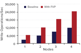


 Fig 1. Write Operations


